 Using the XL-Excellence® Add-In
Location of menu items
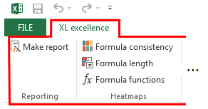
Once installed, the Add-In is usable from two alternate and equivalent menus. The first menu is titled “XL excellence” and is in the main Excel ribbon.
The second menu is in the ADD-INS ribbon.

Function of menu items
Menu items and their functions are detailed below.
- Make report
- Formula consistency
- Formula length
- Formula functions
- Jump from heatmap to source worksheet
- Jump back to heatmap
- Settings
- Share
- About
Make report
This is the main menu item and generates a report on the currently active workbook. The original workbook is not altered and the report appears in a new, separate workbook.
The front page (first tab) of the report looks like this ..

The report includes the following information.
- The version of XL-Excellence® used to generate the report.
- The name and path of the workbook being reported on.
- The name of the user and the date and time.
- A list of cells with errors (there are none in the example above).
- A list of bad names - named ranges that are in error.
- A list of missing tabs - spreadsheet tabs that are on a nominated “required” list but which are absent.
- A list of links to workbooks - references to external workbooks.
- A list of connections to external data sources.
- A list of hyperlinks ‐ one for each tab in the original workbook.
The hyperlinks lead to detailed sub-reports - one for each tab of the original spreadsheet. In the example above the hyperlink "ex1" in the "Structure" section will take the user to a detailed sub-report. Clicking on the hyperlink leads to this tab of the report ..

The sub-report looks much like the corresponding tab in the original spreadsheet (not shown here). But there are some important differences: The colors have been altered. The colors in the report indicate whether the cells in the original spreadsheet had constants or formulae in them. Cells that contained constants are shown in the blue-gray colour and those that had formulae are shown in a tan colour.
As a general design principle constants and formula should be seperate and the colouration in the sub-report gives an overview of how well (or not) this is achieved.
Having hyperlinked to a sub-report we can now use other menu functions for a more in-depth analysis.
Formula consistency
One measure of spreadsheet quality is consistency between formulae. Clicking on the "Formula consistency" menu item will show the consistency (or not) of formulae.
Colours in the report will be updated to show a heatmap colourised on the basis of consistency. Colours will represent formulae. Large areas with the same colour indicate formulas are consistent. Large numbers of small areas with different colours indicate formulas have little consistency. Consider the following example.

In the above heatmap the first block of colours indicate a large amount of inconsistency. In contrast, the second block of colours indicate a large degree of consistency.
Formula length
Clicking on this menu item will regenerate the heatmap. Colours will indicate formula length or complexity..
Consider the following heatmap ..

Colours will be green, orange or red depending on the complexity of the corresponding formulae in the original spreadsheet. Formulae less than a defined length are shown in green, greater than another defined length in red and in-between in orange. [The Settings menu item ‐ see later ‐ is used to define the length thresholds.] “Red” and “orange” formulae are potentially over-complex. Consideration should be given to breaking large complex formulas into smaller, simpler ones.
Formula functions
A small number of Excel functions are “volatile”: Using those functions requires Excel to recalculate the whole workbook even when a single cell changes. This menu item checks whether volatile functions are used in the spreadsheet being reported on. Cells containing formulae that use volatile functions are shown in red. Other functions are shown in green. The volatile functions that can be checked for are: NOW(), TODAY(), OFFSET() and INDIRECT().
The Settings menu item can be used to specify which volatile functions are allowed and which disallowed.
Jump to from heatmap to source worksheet
Use this menu item to jump from a cell in a heatmap to the corresponding cell in the original spreadsheet. This lets you inspect the underlying formulae in the original workbook. Take cell G8 in this example ..
G8's colouration indicates that formulae in row 8 are inconsistent with their neigbouring cells on the same row. To find out why the formulae are inconsistent cell G8 can be selected and then click on the menu item. Selection will transfer to cell G8 in the original spreadsheet ..

The formula in G8 is “=F37/F36-1”. Inspecting the cell to the left — F8 — shows ..

The formula in F8 is “=F36/F35-1”. That formula is inconsistent with the one in G8 because copying and pasting from F8 to G8 would give a different result (=G36/G35-1) to that actually there (=F37/F36-1).
The underlying problem that leads to this inconsistency is that in one part of the spreadsheet dates are in column order and in another they are in row order. To resolve the problem dates should have the same orientation in both sections, or if that cannot be achieved, use the INDEX function in the formulae in row 8 to achieve consistency.
Breaks in colours may indicate inadvertent inconsistencies. Following is an example.

There is a break in colour between cells X55 and Y55. A jump to the source cell of X55 reveals ..

..and the cell to the right – Y55 – reveals ..
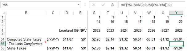
The X55 formula is “=IF(X$1,MIN(0,SUM($F54:X54)),0)” and the Y55 formula is “=IF(Y$1,MIN(0,SUM(F54:Y54)),0)”. The second formula is subtly different: The reference to F54 should actually be to $F54 and is probably an inadvertent formula error.
Jump back to heatmap
This menu item reverses the jump caused by the menu item Jump from heatmap to source worksheet.
In other words: Jump from heatmap to source worksheet takes you from a heatmap to the underlying worksheet. And Jump back to heatmap takes you back to the heatmap from the underlying worksheet.
If you close the original workbook whilst you are examining the report the "jump" functions will no longer work. In other words - both the original spreadsheet and the report need to be kept open for jump to work.
Settings
Use this menu item to set options.
Required tabs

When a report is run a check is made to see whether “required” tabs are found in the workbook being reported on. Missing tabs are listed on the report. The Required tabs page lets you set the names of tabs that should appear in all workbooks that will be reported on.
Formulae

The Formulae tab lets you set thresholds for colours that are reported by the heatmap Formula length menu choice.
Additionally, you can define which formulae are disallowed by the Formula functions menu choice. In the preceding example, formulae containing NOW() or TODAY() will be shown in red. Other functions will be shown in green.
Share
If you wish to share the Add-In with others then press this button. A draft mail will be composed and the Add-In attached to the mail. You can then review the draft, add a list of desired recipients to the “to” and/or “cc” field(s) and then send the mail. (Note - this Sharing feature will work only if you have Outlook mail installed.)
About
Use this menu item to shows the Add-In's version number and installation location. There is also a button to press to check whether a newer version is available to download.
 Next >>